Here is a question I have long wanted to ask:

To use ResNet from torchvision, we can do

import torchvision
model = torchvision.models.ResNet18(pretrained=True).eval()
for p in model.parameters():
    p.requires_grad_(False)

But if we do that, what is our model? And how many of them?

Silly old man! I hear you say.⊕And yes, I spent too much time with accounting recently. That is not healthy. But hear me out.

I will give you a hint when I introduce this by mentioning that in our book, we devote chapter 4, just after we have learned what tensors are, to data representation.

So, one question is: Is the conversion to the data representation part of the model?

One thing that is, sadly, not even part of TorchVision is the list of class names, so we will do our own.

if not os.path.exists('./imagenet_class_index.json'):
    torch.hub.download_url_to_file('https://s3.amazonaws.com/deep-learning-models/image-models/imagenet_class_index.json', 'imagenet_class_index.json', "a1e7a966a1f601d39e4b43e119b3e7dd4a2ad3ea08cf69847cbaf021013767bc")
imagenet_class_index = json.load(open('./imagenet_class_index.json'))
imagenet_classes = [imagenet_class_index[str(i)][1] for i in range(len(imagenet_class_index))]

A missing bit

But back to our question, and let us see what is missing in TorchVision's (and most anyone else's) ResNet.

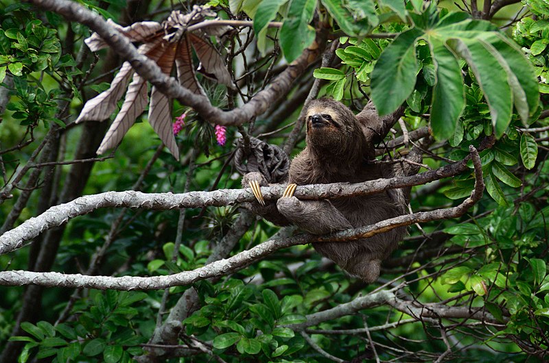
To make things concrete, let us grab an image, and who can resist sloths.⊕CC0-Licensed Image by Kleber Varejão Filho retreived via Wikimedia commons

! wget https://upload.wikimedia.org/wikipedia/commons/thumb/e/e5/Sloth_in_a_tree_%28Unsplash%29.jpg/320px-Sloth_in_a_tree_%28Unsplash%29.jpg

and run it through our model

im = PIL.Image.open('./320px-Sloth_in_a_tree_(Unsplash).jpg')
IPython.display.display(im)
im = torchvision.transforms.functional.to_tensor(im)
pred = model(im[None]).max(1).indices
imagenet_classes[pred]

It says green mamba?! I am not so sure!

If you know TorchVision well or have fallen into this trap yourself, you probably spotted the error: I have not normalized the image. So if we add this, things will be much better:

im2 = torchvision.transforms.functional.normalize(im[None], mean=(0.485, 0.456, 0.406), std=(0.229, 0.224, 0.225))
pred2 = model(im2).max(1).indices
imagenet_classes[pred2]

Three-toed sloth. Much better!

So why do we need to normalize the image? Stemming from the "ImageNet traditions", the data is normalized to have zero mean and unit variance over the ImageNet training dataset. But this normalization is completely model- (or dataset-) specific and the 0 to 1 representation for images seems much more natural (as in occuring in the wild outside computer vision modelling). However, TorchVision's models - like many - don't do this transformation inside the model but leave it to be done in the data preprocessing just like augmentation (which, I will say, is much more independent of the model).

Compare this to typical NLP models in the PyTorch ecosystem: There our models take integer tensors and the embedding layer (which we have as the representation for categorical data per chapter 4) is part of the model. Most of the time, there is another part, though, the conversion to integer tensors and the splitting of the inputs into categorical information, the tokenization, is done in the preprocessing.

Why is this?

The operative answer is because the embedding weights need to be trained while the other bits are fixed transformations. And I have to admit that as a mathematician, it seems hard to find value in defining the tonkenization to be part of the model, except maybe to have a fancy probabilistic model of ambiguous tokenization and then saying "maximum a posteriori" somewhere to go back to the ways we always had.

For images, there seems to be no compelling reason to not do the normalization as a (fixed) initial layer of the model. In this sense, TorchVision's ResNet (and other imagenet) models are incomplete, a bit less of a model than we might expect.

How many models is ResNet?

So far so good. The other interesting part is where does the model we are feeding our images into end in ResNet?

Looking at the overall structure of ResNet, we have the residual blocks with convolutions and shortcuts followed by a pooling layer and then a linear layer (the fully connected part):⊕The visualization is taken from an earlier blog post.

Sometimes people include the (log-) softmax that gives (log-) probabilities in the the model, but the convention in PyTorch seems to not do that and have this integrated into the loss function (typically nn.CrossEntropyLoss, combining LogSoftmax with NLLLoss).

So given that I asked how many models is ResNet, you won't be surprised that I am cutting it up. Specifically, I'll argue that the fully connected layer at the end is a separate second model:

model2 = copy.deepcopy(model)
fc = model2.fc
model2.fc = torch.nn.Identity()

To make things more aligned with what I want to say, I want to take away the bias from the fc layer. Intuitively the bias will roughly give the probabilities of the classes given no information. For ImageNet trained models this is typically pretty uniform (and one can subtract the mean without changing the log-probabilities).

print(f"{fc.bias.min().item():.3f}, {fc.bias.max().item():.3f}")
fc.bias = None # we don't need that, do we?

gives

-0.050, 0.062

So the worst case change is about 0.11 but in typical predictions, the difference between the first and second most likely (according to the model) prediction is much larger. So we drop the bias.⊕The other popular thing about the bias is to consider it as part of the weight and add a fixed 1 input. For example D. MacKay does so in the great Information Theory, Inference, and Learning Algorithms book.

Let us check that it still works:

feat = model2(im2)
preds = fc(feat)
probs = preds.softmax(1)

top_preds = preds.topk(k=5, dim=1)
#pred2_raw.softmax(1)
{imagenet_classes[i]:(i.item(), v.item(), probs[0, i].item()) for i, v in zip(top_preds.indices[0], top_preds.values[0])}

gives

{'three-toed_sloth': (364, 12.637640953063965, 0.7442254424095154),
 'marmoset': (377, 10.666498184204102, 0.10366880148649216),
 'howler_monkey': (379, 9.108072280883789, 0.021818872541189194),
 'macaque': (373, 8.944747924804688, 0.018531112000346184),
 'titi': (380, 8.794718742370605, 0.01594940945506096)}

So indeed, the mormoset prediction has a logit just about 2 smaller than the top one, deleting the bias didn't hurt.

Great, so the linear layer has just a weight and no bias. We can grab the weight and stick it into an embedding layer:

class_emb = torch.nn.Embedding(1000, 512)
with torch.no_grad():
    class_emb.weight.copy_(fc.weight)

This is now a model for the ImageNet 1k categories that, as suggested in our chapter 4, uses the embedding layer.

We can recover the logit score computed above, the following will print tensor([[12.6376]], grad_fn=<MmBackward>).

true_label = torch.tensor([364])
emb = class_emb(true_label)

feat @ emb.t()

and if we wanted to train something, we could compute a loss as

logits = (feat @ class_emb.weight.t())
torch.nn.functional.cross_entropy(logits, true_label)
loss = torch.nn.functional.cross_entropy(logits, true_label)

So in this world, the backbone (the ResBlocks) of ResNet provides an embedding for the images and there is an embedding for the categories. Having these two embeddings is fundamentally very similar to how recommender systems work and also how the venerable Word2Vec embeddings are calculated.

In fact, I can recommend to check out the word2vec paper here: Mikolov et al.: Distributed Representations of Words and Phrases and their Compositionality, NIPS 2013.⊕Note that Mikolov et al. maximize their objective, so they use the negative of our loss functions. I also enjoyed one of the Stanford CS 224d course recordings, but I am not sure which edition.

With word2vec, you have two vectors, the context one and the center one during training (and later have to decide whether to use one of them, the average, or whatever). Just like here. In fact, the above is equivalent to the usual training with ResNet and CrossEntropyLoss but it is also very much like the (1) and (2) formulas of the word2vec paper (except that we don't sum over context vectors).

But this means that if we have many classes and log-softmax followed by NLLLoss stops working - as it does with many classes - we do what word2vec did which is described in their section 2.2: use negative sampling aka noise contrastive estimation (NCE).⊕Note that Mikolov et al. do not claim to have invented it, see their references, but to my mind, they give the formula is more succinctly there then in the cited works and also word2vec has been one of the most influential applications of negative sampling / NCE in this form.

Given an embedding $v_{image}$ of an image and of the $v_{class_i}$ of the classes, instead of the log-softmax and NLLLoss, which we can write as

$$ loss = - (v_{image}^T v_{true\ class}) + \log \sum_i \exp(v_{image}^T v_{class_i}) $$

we take $k$ negative samples and writing $\sigma$ for the Sigmoid function we compute as in Mikolov et al's equation (4):

$$ loss = - \log \sigma (v_{image}^T v_{true\ class}) - \sum_{i=1}^k \log \sigma(- v_{image}^T v_{c_i}) $$ where $c_i$ is randomly sampled (uniform perhaps for us) from the negative classes.

If we do not want repetitions (nor the true class) in our negative sampling, we might write this in PyTorch as

neg_k = 5
batch_size = 1
num_classes = 1000
probs = torch.ones(batch_size, num_classes - 1)

# this gives us non-repeating false labels
rnd = torch.multinomial(probs, neg_k, replacement=False)
rnd += (rnd >= true_label)

pos_logit = torch.gather(logits, 1, true_label[:, None])
neg_logit = torch.gather(logits, 1, rnd)

nce_loss = -torch.nn.functional.logsigmoid(pos_logit) - torch.nn.functional.logsigmoid(-neg_logit).sum(1)

Of course, we might implement negative sampling directly on the logits as output by the ResNet model as is, too, and in practice we would. But personally, everything is an embedding helps me only remember how things are done once.

Other ideas for that category embedding

I briefly want to mention two things that seem very natural now:

• E. Hoffer et al. Fix your classifier: ... propose to fix the embeddings.
• A. Frome et. al. DeViSE essentially suggest to train the backbone to predict word vectors (I think there are additional linear layers above the convolutions, but still).
• Unsupervised / Self-supervised learning is essentially trying to train only the backbone (of course, the difficult part is how to do this), and evaluation is often done by seeing if category embeddings can be constructed that fit that backbone well.

Limitations of the two embedding thinking

Sadly, this isn't the one thing that explains everything (or all of what I have written above would have been said by much smarter people prominently enough for me to take note and not bore you with a rehash).

One immediate limitation is that this only applies to models with a single linear layer at the top. If there are several, what is the category embedding?

If we look at the venerable VGG models (TorchVision provides both the original and the variant including batch norm layers and we use the latter), we have the features submodule consisting of convolutions, relu, batch norm, and pooling layers and then the classifier, which has three linear layers:

vgg = torchvision.models.vgg19_bn(pretrained=True).eval()
vgg.classifier

gives

Sequential(
  (0): Linear(in_features=25088, out_features=4096, bias=True)
  (1): ReLU(inplace=True)
  (2): Dropout(p=0.5, inplace=False)
  (3): Linear(in_features=4096, out_features=4096, bias=True)
  (4): ReLU(inplace=True)
  (5): Dropout(p=0.5, inplace=False)
  (6): Linear(in_features=4096, out_features=1000, bias=True)
)

Obviously, we cannot just cleverly invert this. To get some idea what we need here, we go back to the single linear layer as it sits on top of ResNet. It takes the space in which the image embeddings computed by the backbone lie and maps each point to a vector of class scores (and when applying softmax also to the class probabilities). If we always pick the maximum score / probability and neglect the uncertainty information, we get decision boundaries in this embedding space.

For a single linear layer without bias, these are sectors of the space around the origin (this is because when we multiply an input vector $v$ with a positive scalar $\lambda$, the index of the largest element remains the same). So this picture is how it generically looks like:

N = 100
l = torch.nn.Linear(2, 4, bias=False)
xx = torch.linspace(-extend, extend, N)[None, :].expand(N, N)
yy = torch.linspace(-extend, extend, N)[:, None].expand(N, N)
inps = torch.zeros(N, N, 2)
zz = torch.stack([xx, yy], -1)
res = (l(zz).argmax(-1))
pyplot.imshow(res)
pyplot.axis('off')

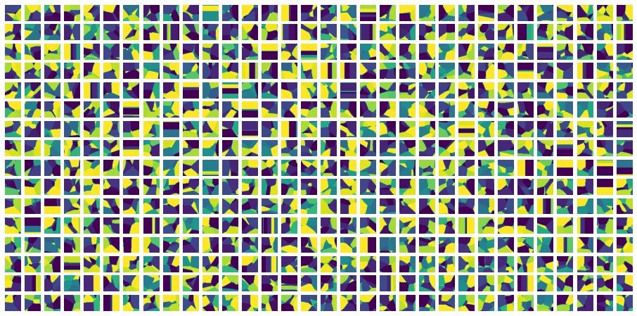
But having multiple layers, these decision regions become much more elaborate, as we can see looking at the last two layers in the VGG model:

import matplotlib

vgg = torchvision.models.vgg19_bn(pretrained=True).eval()
top = vgg.classifier[3:]
with torch.no_grad():
    top[-1].bias.zero_()


extend = 4
N = 50
Mx = 32
My = 16
pyplot.figure(figsize=(16, 8))
for i in range(My):
  print("\r", i, end="")
  for j in range(Mx):
    ij = i * Mx + j + 1
    xx = torch.linspace(-extend, extend, N)[None, :].expand(N, N)
    yy = torch.linspace(-extend, extend, N)[:, None].expand(N, N)
    inps = torch.zeros(N, N, 4096)
    zz = torch.stack([xx, yy], -1)
    inps[:, :, ij * 2: ij * 2 + 2] = zz
    res = (top(inps).argmax(-1))
    pyplot.subplot(My, Mx, ij)
    pyplot.imshow(res)
    pyplot.axis('off')

gives this pictures (of many decision regions along two input dimensions) where we clearly see curved decision boundaries:

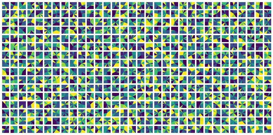
As an aside: One thing not to be fooled from is that the untrained top does not show curved boundaries much. Using pretrained=False above we get:

So here we are.

Of course, people have done various things to get a different view on the more elaborate decision regions. My favourite ones probably are metric / prototypical learning approaches and the closely related Gaussian processes as classification heads. But all this is for another blog post.

Conclusion

So we looked at ResNet and - not entirely in earnest - found that it is almost two models. Still I hope that some of the lines of thought presented here help with intuiting about deep learning models and how they are applied.

I hope you enjoyed this little look at ResNet. I look forward to your feedback and comments at tv@lernapparat.de.

I do Machine Learning and PyTorch training and consulting at MathInf GmbH. Check it out if you need help with your modelling.